Estimating Uncertainty in Machine Learning Models — Part 1
“We demand rigidly defined areas of doubt and uncertainty!”
– Douglas Adams, The Hitchhiker’s Guide to the Galaxy
Why is uncertainty important?
Let’s imagine for a second that we’re building a computer vision model for a construction company, ABC Construction. The company is interested in automating its aerial site surveillance process, and would like our algorithm to run on their drones.
We happily get to work, and deploy our algorithm onto their fleets of drones, and go home thinking that the project is a great success. A week later, we get a call from ABC Construction saying that the drones keep crashing into the white trucks that they have parked on all their sites. You rush to one of the sites to examine the vision model, and realize that it is mistakenly predicting that the side of the white truck is just the bright sky. Given this single prediction, the drones are flying straight into the trucks, thinking that there is nothing there.
When making predictions about data in the real world, it’s a good idea to include an estimate of how sure your model is about its predictions. This is especially true if models are required to make decisions that have real consequences to peoples lives. In applications such as self driving cars, health care, insurance, etc, measures of uncertainty can help prevent serious accidents from happening.
Sources of uncertainty
When modeling any process, we are primarily concerned with two types of uncertainty.
Aleatoric Uncertainty: This is the uncertainty that is inherent in the process we are trying to explain. e.g. A ping pong ball dropped from the same location above a table will land in a slightly different spot every time, due to complex interactions with the surrounding air. Uncertainty in this category tends to be irreducible in practice.
Epistemic Uncertainty: This is the uncertainty attributed to an inadequate knowledge of the model most suited to explain the data. This uncertainty is reducible given more knowledge about the problem at hand. e.g. reduce this uncertainty by adding more parameters to the model, gather more data etc.
So how do we estimate uncertainty?
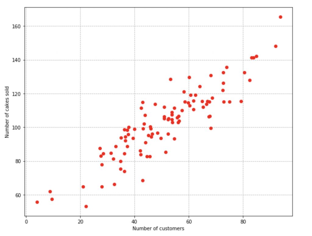
Let’s consider the case of a bakery trying to estimate the number of cakes it will sell in a given month based on the number of customers that enter the bakery. We’re going to try and model this problem using a simple linear regression model. We will then try to estimate the different types of epistemic uncertainty in this model from the available data that we have.

The coefficients of this model are subject to sampling uncertainty, and it is unlikely that we will ever determine the true parameters of the model from the sample data. Therefore, providing an estimate of the set of possible values for these coefficients will inform us of how appropriately our current model is able to explain the data.
First, lets generate some data. We’re going to sample our x values from a scaled and shifted unit normal distribution. Our y values are just perturbations of these x values.
import numpy as np

from numpy.random import randn, randint
from numpy.random import seed

# random number seed
seed(1)

# Number of samples
size = 100

x = 20 * (2.5 + randn(size))
y = x + (10 * randn(size) + 50)
Our resulting data ends up looking like this
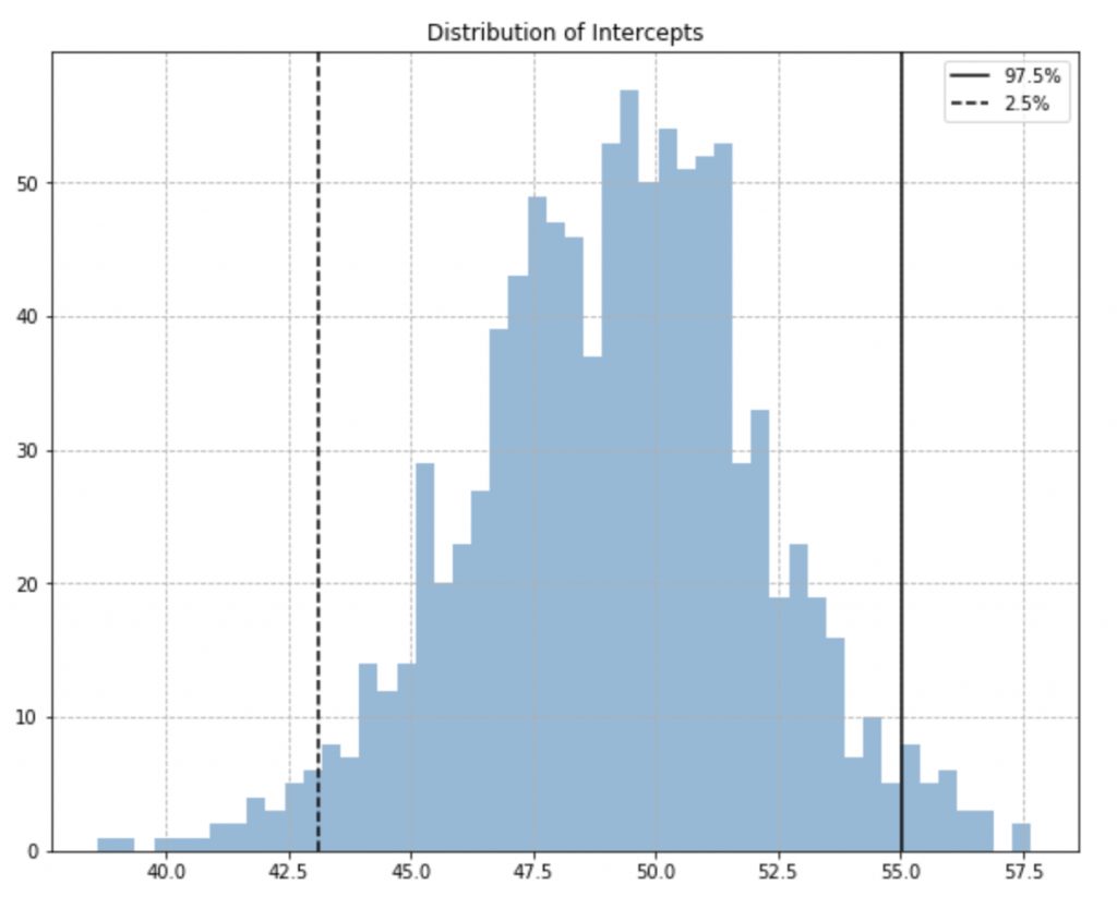
We’re going to start with estimating the uncertainty in our model parameters using bootstrap sampling. Bootstrap sampling is a technique to build new datasets by sampling with replacement from the original dataset. It generates variants of our dataset, and can give us some intuition into the range of parameters that could describe the data.
In the code below, we run 1000 iterations of bootstrap sampling, fit a linear regression model to each sample dataset, and log the coefficients, and intercepts of the model at every iteration.
from sklearn.utils import resample

coefficients = []
intercepts = []

for _ in range(1000):
    idx = randint(0, size, size)
    x_train = x[idx]
    y_train = y[idx]

    model = LinearRegression().fit(x_train, y_train)

    coefficients.append(model.coef_.item())
    intercepts.append(model.intercept_)
Finally, we extract the 97.5th, 2.5th percentile from the logged coefficients. This gives us the 95% confidence interval of the coefficients and intercepts. Using percentiles to determine the interval has the added advantage of not making assumptions about the sampling distribution of the coefficients.
upper_coefficient = np.percentile(coefficients, 97.5)
upper_intercept = np.percentile(intercepts, 97.5)

lower_coefficient = np.percentile(coefficients, 2.5)
lower_intercept = np.percentile(intercepts, 2.5)

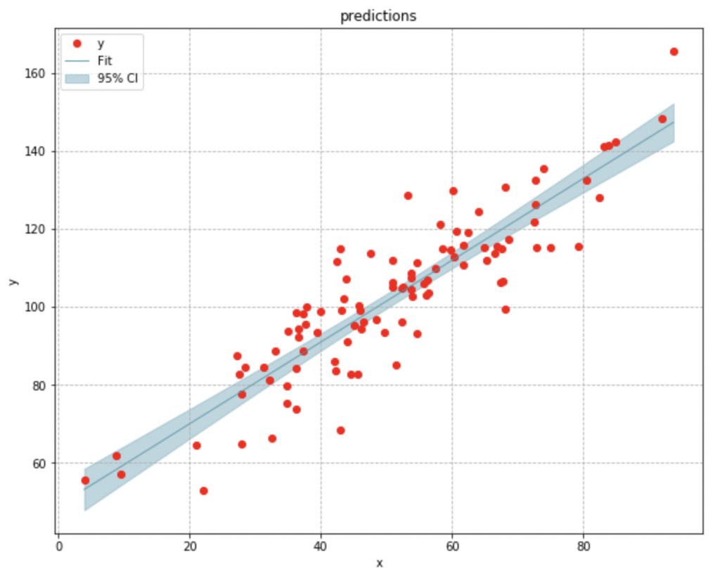
We can now use these coefficients to plot the 95% confidence interval for a family of curves that can describe the data.
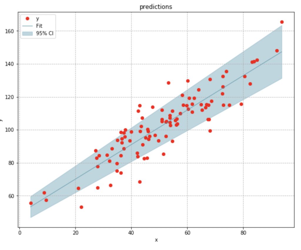
Now lets estimate the uncertainty in the models predictions. Our linear regression model is predicting the mean number of cakes sold given the fact that x number of customers have come in to the store. We expect different values of x to produce different mean responses in y, and we’re going to assume that for a fixed x, the response y, is normally distributed.
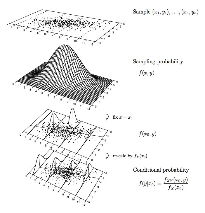
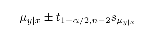
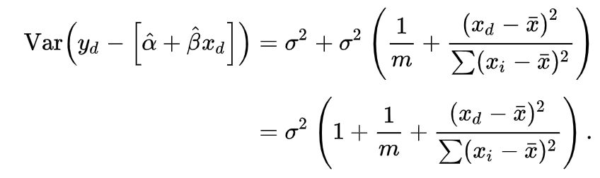
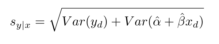
Based on this assumption, we can approximate the variance in y conditioned on x, using the residuals from our predictions. With this variance in hand, we can calculate the standard error of the mean response, and use that to build the confidence interval of the mean response. This is a measure of how well we are approximating the true mean response of y. The smaller we can make this value, the better.
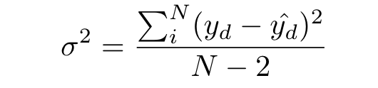

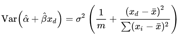
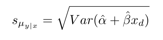
The variance in our conditional mean is dependent on the variance in our coefficient and intercept. The standard error is just the square root of this variance. Since the standard error of the conditional mean is proportional to the deviation in the values of x from themean, we can see it getting narrower as it approaches the mean value of x.
With the confidence interval, the bakery is able to determine the interval for the average number of cakes it will sell for a given number of customers, however, they still do not know the interval for the number possible of cakes they might sell for a given number of customers.
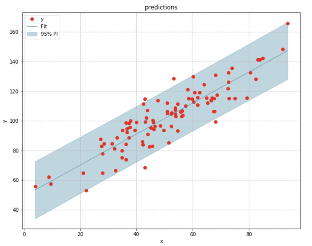
A confidence interval only accounts for drift in the mean response of y. It does not provide the interval for all possible values of y for a given x value. In order to do that, we would need to use a prediction interval.
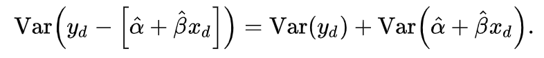
The prediction interval derived in a similar manner as the confidence interval. The only difference is that we include the variance of our dependent variable y when calculating the standard error, which leads to a wider interval.
Conclusion
In the first part of our series on estimating uncertainty, we looked at ways to estimate sources of epistemic uncertainty in a simple regression model. Of course, these estimations become a lot harder when the size and complexity of your data, and model increase.
Bootstrapping techniques won’t work when we’re dealing with large neural networks, and estimating the confidence and prediction intervals through the standard error only works when normality assumptions are made about the sampling distributions of the model’s residuals, and parameters. How do we measure uncertainty when these assumptions are violated?
In the next part of this series we will looks at ways to quantify uncertainty in more complex models.
Related Articles

